The only way to deal with that data is to split a cell in Excel. There are different ways to do this, depending on the format of the data. In this article you’ll learn how to split a cell, how to roll that out to an entire column, and when you should choose each option.
Convert Text To Columns
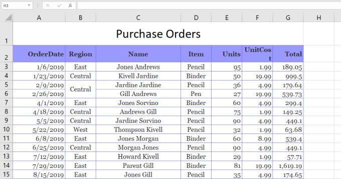
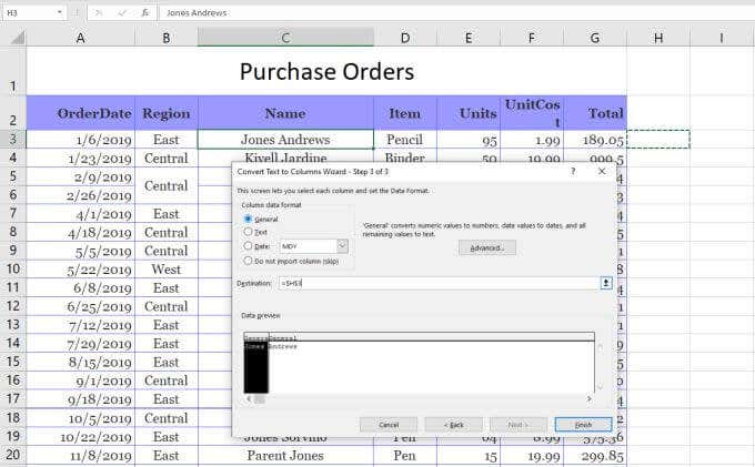
One of the most common methods to split a cell in Excel is using the Text to Columns tool. This lets you split an entire column of cells using whatever rules you like. The feature also includes an easy-to-use wizard, which is why most people prefer using it. It also handles any text format, whether the separating text is a space, a tab, or a comma. Let’s look at an example of how to use the Text to Columns feature in Excel. In this example, we want to split the Name column into two cells, the first name and the last name of the salesperson. To do this:
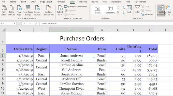
- Select the Data menu. Then select Text to Columns in the Data Tools group on the ribbon.
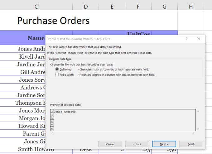
- This will open a three-step wizard. In the first window, make sure Delimited is selected and select Next.
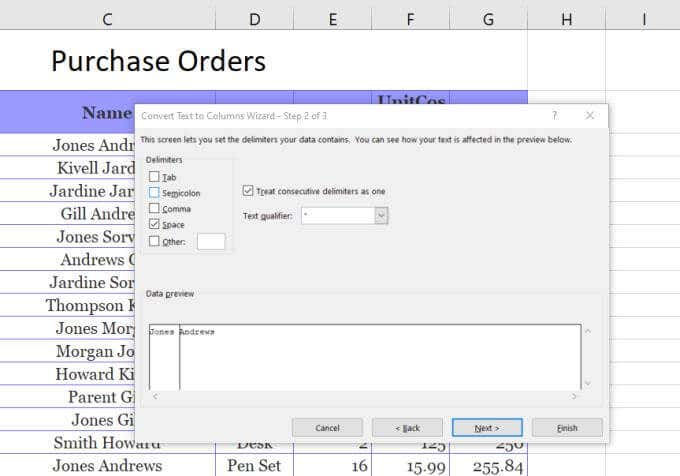
- On the next Wizard window, deselect Tab and make sure Space is selected. Select Next to continue.
- On the next window, select the Destination field. Then, in the spreadsheet, select the cell where you want the first name to go. This will update the cell in the Destination field to where you’ve selected.
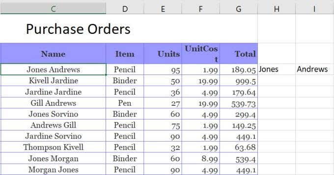
- Now, select Finish to complete the Wizard. You’ll see that the single cell that contained both the first name and last name has been split into two cells that contain each one individually. Note: The process above works because the data to split in the cell had a space separating the text. This text-to-column feature can also handle splitting a cell in Excel if the text is separated by a tab, semicolon, comma, or any other character you specify.
Use Excel Text Functions
Another way to split a cell in Excel is by using different text functions. Text functions let you extract pieces of a cell that you can output into another cell. Text functions in Excel include:
Left(): Extract a number of characters from the left side of the textRight(): Extract a number of characters from the right side of the textMid(): Extract a number of characters from the middle of a stringFind(): Find a substring inside of another stringLen(): Return the total number of characters in a string of text
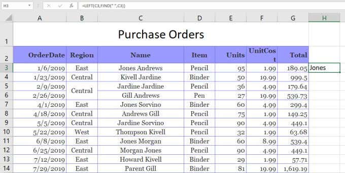
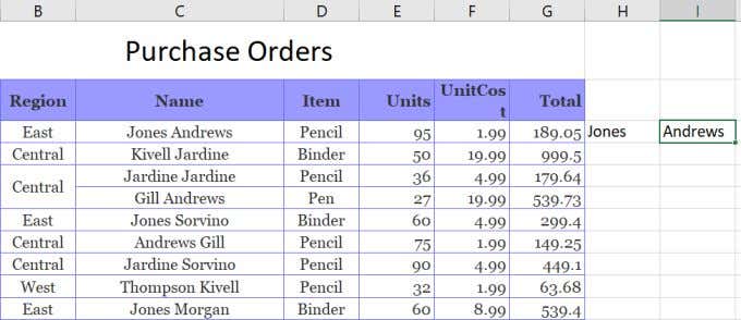
To split cells, you may not need to use all of these functions. However, there are multiple ways you can use these to accomplish the same thing. For example, you can use the Left and Find function to extract the first name. The Find function helps because it can tell you where the delimiting character is. In this case, it’s a space. So the function would look like this: =LEFT(C3,FIND(” “,C3)) When you press enter after typing this function, you’ll see that the first name is extracted from the string in cell C3. This works, because the Left function needs the number of characters to extract. Since the space character is positioned at the end of the first name, you can use the FIND function to find the space, which returns the number of characters you need to get the first name. You can extract the last name either using either the Right function or the Mid function. To use the Right function: =RIGHT(C3,LEN(C3)-FIND(” “,C3)) This will extract the last name by finding the position of the space, then subtracting that from the length of the total string. This gives the Right function the number of characters it needs to extract the last name. Technically, you could do the same thing as the Right function using the Mid function, like this: =MID(C3,FIND(” “,C3),LEN(C3)-FIND(” “,C3)) In this case the Find function gives the Mid function the starting point, and the Len combined with Find provides the number of characters to extract. This will also return the last name. Using Excel text functions to split a cell in Excel works as well as the Text-To-Column solution, but it also lets you fill the entire column beneath those results using the same functions.
Split Cell in Excel Using Flash Fill
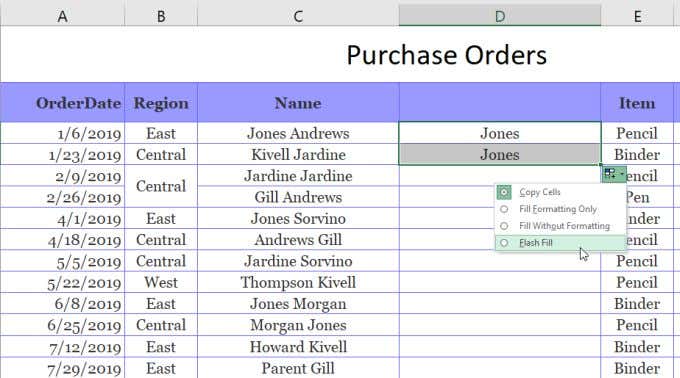
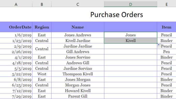
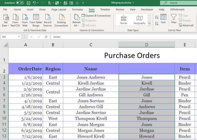
The last option to split a cell in Excel is using the Flash Fill feature. This requires that the cells you’re splitting the original one into are right beside it. If this is the case, all you have to do is type the part of the original cell that you want to split out. Then drag the lower right corner of the cell down to fill the cell beneath it. When you do this, you’ll see a small cell fill icon appear with a small plus sign next to it. Select this icon and you’ll see a menu pop-up. Select Flash Fill in this menu. When you do this, you’ll see that the Flash Fill feature automatically detects why you typed what you typed, and will repeat the process in the next cell. It’ll do this by detecting and filling in the first name in the original cell to the left. You can actually do this same procedure when you fill the entire column. Select the same icon and select Flash Fill. It’ll fill the entire column with the correct first name from the cells to the left. You can then copy this entire column and paste it into another column, then repeat this same process to extract the last names. Finally, copy and paste that entire column where you want it to go in the spreadsheet. Then delete the original column you used to perform the Flash Fill process.
Splitting Cells in Excel
As you can see there are a few ways to accomplish the same thing. How you split a cell in Excel boils down to where you want the final result to go and what you plan to do with it. Any options works, so choose the one that makes the most sense for your situation and use it.
